Effect size: Difference between revisions
| Line 317: | Line 317: | ||
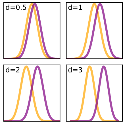
For Cohen's ''d'' an effect size of 0.2 to 0.3 might be a "small" effect, around 0.5 a "medium" effect and 0.8 to infinity, a "large" effect.<ref name="CohenJ1988Statistical"/>{{Rp|25|date=November 2012}} |
For Cohen's ''d'' an effect size of 0.2 to 0.3 might be a "small" effect, around 0.5 a "medium" effect and 0.8 to infinity, a "large" effect.<ref name="CohenJ1988Statistical"/>{{Rp|25|date=November 2012}} |
||
(But |
(But the ''d'' might be larger than one.) |
||
Cohen's text<ref name="CohenJ1988Statistical"/> anticipates Lenth's concerns: |
Cohen's text<ref name="CohenJ1988Statistical"/> anticipates Lenth's concerns: |
||
Revision as of 01:29, 1 February 2014
This article needs attention from an expert in statistics. Please add a reason or a talk parameter to this template to explain the issue with the article. (May 2011) |
In statistics, an effect size is a measure of the strength of a phenomenon[1] (for example, the change in an outcome after experimental intervention). An effect size calculated from data is a descriptive statistic that conveys the estimated magnitude of a relationship without making any statement about whether the apparent relationship in the data reflects a true relationship in the population. In that way, effect sizes complement inferential statistics such as p-values. Among other uses, effect size measures play an important role in meta-analysis studies that summarize findings from a specific area of research, and in statistical power analyses.
The concept of effect size already appears in everyday language. For example, a weight loss program may boast that it leads to an average weight loss of 30 pounds. In this case, 30 pounds is the claimed effect size. Another example is that a tutoring program may claim that it raises school performance by one letter grade. This grade increase is the claimed effect size of the program. These are both examples of "absolute effect sizes", meaning that they convey the average difference between two groups without any discussion of the variability within the groups. For example, if the weight loss program results in an average loss of 30 pounds, it is possible that every participant loses exactly 30 pounds, or half the participants lose 60 pounds and half lose no weight at all.
Reporting effect sizes is considered good practice when presenting empirical research findings in many fields.[2][3] The reporting of effect sizes facilitates the interpretation of the substantive, as opposed to the statistical, significance of a research result.[4] Effect sizes are particularly prominent in social and medical research. Relative and absolute measures of effect size convey different information, and can be used complementarily. A prominent task force in the psychology research community expressed the following recommendation:
Always present effect sizes for primary outcomes...If the units of measurement are meaningful on a practical level (e.g., number of cigarettes smoked per day), then we usually prefer an unstandardized measure (regression coefficient or mean difference) to a standardized measure (r or d).
— L. Wilkinson and APA Task Force on Statistical Inference (1999, p. 599)
Overview
Population and sample effect sizes
The term effect size can refer to a statistic calculated from a sample of data, or to a parameter of a hypothetical statistical population. Conventions for distinguishing sample from population effect sizes follow standard statistical practices — one common approach is to use Greek letters like ρ to denote population parameters and Latin letters like r to denote the corresponding statistic; alternatively, a "hat" can be placed over the population parameter to denote the statistic, e.g. with being the estimate of the parameter .
As in any statistical setting, effect sizes are estimated with error, and may be biased unless the effect size estimator that is used is appropriate for the manner in which the data were sampled and the manner in which the measurements were made. An example of this is publication bias, which occurs when scientists only report results when the estimated effect sizes are large or are statistically significant. As a result, if many researchers are carrying out studies under low statistical power, the reported results are biased to be stronger than true effects, if any.[5] Another example where effect sizes may be distorted is in a multiple trial experiment, where the effect size calculation is based on the averaged or aggregated response across the trials.[6]
Relationship to test statistics
Sample-based effect sizes are distinguished from test statistics used in hypothesis testing, in that they estimate the strength of an apparent relationship, rather than assigning a significance level reflecting whether the relationship could be due to chance. The effect size does not determine the significance level, or vice-versa. Given a sufficiently large sample size, a statistical comparison will always show a significant difference unless the population effect size is exactly zero. For example, a sample Pearson correlation coefficient of 0.1 is strongly statistically significant if the sample size is 1000. Reporting only the significant p-value from this analysis could be misleading if a correlation of 0.1 is too small to be of interest in a particular application.
Standardized and unstandardized effect sizes
The term effect size can refer to a standardized measures of effect (such as r, Cohen's d, and odds ratio), or to an unstandardized measure (e.g., the raw difference between group means and unstandardized regression coefficients). Standardized effect size measures are typically used when the metrics of variables being studied do not have intrinsic meaning (e.g., a score on a personality test on an arbitrary scale), when results from multiple studies are being combined, when some or all of the studies use different scales, or when it is desired to convey the size of an effect relative to the variability in the population. In meta-analysis, standardized effect sizes are used as a common measure that can be calculated for different studies and then combined into an overall summary.
Types
Effect sizes based on "variance explained"
These effect sizes estimate the amount of the variance within an experiment that is "explained" or "accounted for" by the experiment's model.
Pearson r (correlation)
Pearson's correlation, often denoted r and introduced by Karl Pearson, is widely used as an effect size when paired quantitative data are available; for instance if one were studying the relationship between birth weight and longevity. The correlation coefficient can also be used when the data are binary. Pearson's r can vary in magnitude from −1 to 1, with −1 indicating a perfect negative linear relation, 1 indicating a perfect positive linear relation, and 0 indicating no linear relation between two variables. Cohen gives the following guidelines for the social sciences:[7][8]
| Effect size | r |
|---|---|
| Small | 0.10 |
| Medium | 0.30 |
| Large | 0.50 |
Coefficient of determination
A related effect size is r², the coefficient of determination (also referred to as "r-squared"), calculated as the square of the Pearson correlation r. In the case of paired data, this is a measure of the proportion of variance shared by the two variables, and varies from 0 to 1. For example, with an r of 0.21 the coefficient of determination is 0.0441, meaning that 4.4% of the variance of either variable is shared with the other variable. The r² is always positive, so does not convey the direction of the correlation between the two variables.
Eta-squared, η2
Eta-squared describes the ratio of variance explained in the dependent variable by a predictor while controlling for other predictors, making it analogous to the r2. Eta-squared is a biased estimator of the variance explained by the model in the population (it estimates only the effect size in the sample). This estimate shares the weakness with r2 that each additional variable will automatically increase the value of η2. In addition, it measures the variance explained of the sample, not the population, meaning that it will always overestimate the effect size, although the bias grows smaller as the sample grows larger.
Omega-squared, ω2
Template:See also subsection A less biased estimator of the variance explained in the population is ω2[9][10][11]
This form of the formula is limited to between-subjects analysis with equal sample sizes in all cells,.[11] Since it is less biased (although not unbiased), ω2 is preferable to η2; however, it can be more inconvenient to calculate for complex analyses. A generalized form of the estimator has been published for between-subjects and within-subjects analysis, repeated measure, mixed design, and randomized block design experiments.[12] In addition, methods to calculate partial Omega2 for individual factors and combined factors in designs with up to three independent variables have been published.[12]
Cohen's ƒ2
Cohen's ƒ2 is one of several effect size measures to use in the context of an F-test for ANOVA or multiple regression. Its amount of bias (overestimation of the effect size for the ANOVA) depends on the bias of its underlying measurement of variance explained (e.g., R2, η2, ω2).
The ƒ2 effect size measure for multiple regression is defined as:
- where R2 is the squared multiple correlation.
Likewise, ƒ2 can be defined as:
- or
- for models described by those effect size measures.[13]
The effect size measure for hierarchical multiple regression is defined as:
- where R2A is the variance accounted for by a set of one or more independent variables A, and R2AB is the combined variance accounted for by A and another set of one or more independent variables B. By convention, ƒ2A effect sizes of 0.02, 0.15, and 0.35 are termed small, medium, and large, respectively.[7]
Cohen's can also be found for factorial analysis of variance (ANOVA, aka the F-test) working backwards using :
In a balanced design (equivalent sample sizes across groups) of ANOVA, the corresponding population parameter of is
wherein μj denotes the population mean within the jth group of the total K groups, and σ the equivalent population standard deviations within each groups. SS is the sum of squares manipulation in ANOVA.
Effect sizes based on means or distances between/among means
This article needs attention from an expert in Statistics. Please add a reason or a talk parameter to this template to explain the issue with the article. (March 2011) |
A (population) effect size θ based on means usually considers the standardized mean difference between two populations[14]: 78
where μ1 is the mean for one population, μ2 is the mean for the other population, and σ is a standard deviation based on either or both populations.
In the practical setting the population values are typically not known and must be estimated from sample statistics. The several versions of effect sizes based on means differ with respect to which statistics are used.
This form for the effect size resembles the computation for a t-test statistic, with the critical difference that the t-test statistic includes a factor of . This means that for a given effect size, the significance level increases with the sample size. Unlike the t-test statistic, the effect size aims to estimate a population parameter, so is not affected by the sample size.
Cohen's d
Cohen's d is defined as the difference between two means divided by a standard deviation for the data, i.e.,
Cohen's d is frequently used in estimating sample sizes. A lower Cohen's d indicates the necessity of larger sample sizes, and vice versa, as can subsequently be determined together with the additional parameters of desired significance level and statistical power.[15]
What precisely the standard deviation s is was not originally made explicit by Jacob Cohen because he defined it (using the symbol "σ") as "the standard deviation of either population (since they are assumed equal)".[7]: 20 Other authors make the computation of the standard deviation more explicit with the following definition for a pooled standard deviation[16]: 14 with two independent samples.
This definition of "Cohen's d" is termed the maximum likelihood estimator by Hedges and Olkin,[14] and it is related to Hedges's g by a scaling factor (see below).
So, in the example above of visiting England and observing men's and women's heights, the data (Aaron,Kromrey,& Ferron, 1998, November; from a 2004 UK representative sample of 2436 men and 3311 women) are:
- Men: mean height = 1750 mm; standard deviation = 89.93 mm
- Women: mean height = 1612 mm; standard deviation = 69.05 mm
The effect size (using Cohen's d) would equal 1.72 (95% confidence intervals: 1.66 – 1.78). This is very large and you should have no problem in detecting that there is a consistent height difference, on average, between men and women.
Glass's Δ
In 1976 Gene V. Glass proposed an estimator of the effect size that uses only the standard deviation of the second group[14]: 78
The second group may be regarded as a control group, and Glass argued that if several treatments were compared to the control group it would be better to use just the standard deviation computed from the control group, so that effect sizes would not differ under equal means and different variances.
Under a correct assumption of equal population variances a pooled estimate for σ is more precise.
Hedges's g
Hedges's g, suggested by Larry Hedges in 1981,[17] is like the other measures based on a standardized difference[14]: 79
but its pooled standard deviation is computed slightly differently from Cohen's d. Initially, one can calculate the pooled standard deviation as if doing so for Cohen's d:
However, as an estimator for the population effect size θ it is biased. Nevertheless, this bias can be approximately corrected through multiplication by a factor
Hedges and Olkin refer to this less-biased estimator as d,[14] but it is not the same as Cohen's d. The exact form for the correction factor J() involves the gamma function[14]: 104
Ψ, Root-Mean-Square Standardized Effect
A similar effect size estimator for multiple comparisons (e.g., ANOVA) is the Ψ root-mean-square standardized effect.[13] This essentially presents the omnibus difference of the entire model adjusted by the root mean square, analogous to d or g. The simplest formula for Ψ, suitable for one-way ANOVA, is
In addition, a generalization for multi-factorial designs has been provided.[13]
Distribution of effect sizes based on means
Provided that the data is Gaussian distributed a scaled Hedges's g, , follows a noncentral t-distribution with the noncentrality parameter and (n1 + n2 − 2) degrees of freedom. Likewise, the scaled Glass's Δ is distributed with n2 − 1 degrees of freedom.
From the distribution it is possible to compute the expectation and variance of the effect sizes.
In some cases large sample approximations for the variance are used. One suggestion for the variance of Hedges's unbiased estimator is[14]: 86
Effect sizes for associations among categorical variables
|
|
|
| Phi (φ) | Cramér's V (φc) |
|---|
Commonly used measures of association for the chi-squared test are the Phi coefficient and Cramér's V (sometimes referred to as Cramér's phi and denoted as φc). Phi is related to the point-biserial correlation coefficient and Cohen's d and estimates the extent of the relationship between two variables (2 x 2).[18] Cramér's V may be used with variables having more than two levels.
Phi can be computed by finding the square root of the chi-squared statistic divided by the sample size.
Similarly, Cramér's V is computed by taking the square root of the chi-squared statistic divided by the sample size and the length of the minimum dimension (k is the smaller of the number of rows r or columns c).
φc is the intercorrelation of the two discrete variables[19] and may be computed for any value of r or c. However, as chi-squared values tend to increase with the number of cells, the greater the difference between r and c, the more likely V will tend to 1 without strong evidence of a meaningful correlation.
Cramér's V may also be applied to 'goodness of fit' chi-squared models (i.e. those where c=1). In this case it functions as a measure of tendency towards a single outcome (i.e. out of k outcomes). In such a case one must use r for k, in order to preserve the 0 to 1 range of V. Otherwise, using c would reduce the equation to that for Phi.
Odds ratio
The odds ratio (OR) is another useful effect size. It is appropriate when the research question focuses on the degree of association between two binary variables. For example, consider a study of spelling ability. In a control group, two students pass the class for every one who fails, so the odds of passing are two to one (or 2/1 = 2). In the treatment group, six students pass for every one who fails, so the odds of passing are six to one (or 6/1 = 6). The effect size can be computed by noting that the odds of passing in the treatment group are three times higher than in the control group (because 6 divided by 2 is 3). Therefore, the odds ratio is 3. Odds ratio statistics are on a different scale than Cohen's d, so this '3' is not comparable to a Cohen's d of 3.
Relative risk
The relative risk (RR), also called risk ratio, is simply the risk (probability) of an event relative to some independent variable. This measure of effect size differs from the odds ratio in that it compares probabilities instead of odds, but asymptotically approaches the latter for small probabilities. Using the example above, the probabilities for those in the control group and treatment group passing is 2/3 (or 0.67) and 6/7 (or 0.86), respectively. The effect size can be computed the same as above, but using the probabilities instead. Therefore, the relative risk is 1.28. Since rather large probabilities of passing were used, there is a large difference between relative risk and odds ratio. Had failure (a smaller probability) been used as the event (rather than passing), the difference between the two measures of effect size would not be so great.
While both measures are useful, they have different statistical uses. In medical research, the odds ratio is commonly used for case-control studies, as odds, but not probabilities, are usually estimated.[20] Relative risk is commonly used in randomized controlled trials and cohort studies.[21] When the incidence of outcomes are rare in the study population (generally interpreted to mean less than 10%), the odds ratio is considered a good estimate of the risk ratio. However, as outcomes become more common, the odds ratio and risk ratio diverge, with the odds ratio overestimating or underestimating the risk ratio when the estimates are greater than or less than 1, respectively. When estimates of the incidence of outcomes are available, methods exist to convert odds ratios to risk ratios.[22][23]
Confidence intervals by means of noncentrality parameters
Confidence intervals of standardized effect sizes, especially Cohen's and , rely on the calculation of confidence intervals of noncentrality parameters (ncp). A common approach to construct the confidence interval of ncp is to find the critical ncp values to fit the observed statistic to tail quantiles α/2 and (1 − α/2). The SAS and R-package MBESS provides functions to find critical values of ncp.
For a single group, M denotes the sample mean, μ the population mean, SD the sample's standard deviation, σ the population's standard deviation, and n is the sample size of the group. The t value is used to test the hypothesis on the difference between the mean and a baseline μbaseline. Usually, μbaseline is zero. In the case of two related groups, the single group is constructed by the differences in pair of samples, while SD and σ denote the sample's and population's standard deviations of differences rather than within original two groups.
and Cohen's
is the point estimate of
So,
t-test for mean difference between two independent groups
n1 or n2 are the respective sample sizes.
wherein
and Cohen's
- is the point estimate of
So,
One-way ANOVA test for mean difference across multiple independent groups
One-way ANOVA test applies noncentral F distribution. While with a given population standard deviation , the same test question applies noncentral chi-squared distribution.
For each j-th sample within i-th group Xi,j, denote
While,
So, both ncp(s) of F and equate
In case of for K independent groups of same size, the total sample size is N := n·K.
The t-test for a pair of independent groups is a special case of one-way ANOVA. Note that the noncentrality parameter of F is not comparable to the noncentrality parameter of the corresponding t. Actually, , and .
"Small", "medium", "large" effect sizes
Some fields using effect sizes apply words such as "small", "medium" and "large" to the size of the effect. Whether an effect size should be interpreted small, medium, or large depends on its substantive context and its operational definition. Cohen's conventional criteria small, medium, or big[7] are near ubiquitous across many fields. Power analysis or sample size planning requires an assumed population parameter of effect sizes. Many researchers adopt Cohen's standards as default alternative hypotheses. Russell Lenth [sic] criticized them as T-shirt effect sizes.[24]
This is an elaborate way to arrive at the same sample size that has been used in past social science studies of large, medium, and small size (respectively). The method uses a standardized effect size as the goal. Think about it: for a "medium" effect size, you'll choose the same n regardless of the accuracy or reliability of your instrument, or the narrowness or diversity of your subjects. Clearly, important considerations are being ignored here. "Medium" is definitely not the message!
For Cohen's d an effect size of 0.2 to 0.3 might be a "small" effect, around 0.5 a "medium" effect and 0.8 to infinity, a "large" effect.[7]: 25 (But the d might be larger than one.)
Cohen's text[7] anticipates Lenth's concerns:
"The terms 'small,' 'medium,' and 'large' are relative, not only to each other, but to the area of behavioral science or even more particularly to the specific content and research method being employed in any given investigation....In the face of this relativity, there is a certain risk inherent in offering conventional operational definitions for these terms for use in power analysis in as diverse a field of inquiry as behavioral science. This risk is nevertheless accepted in the belief that more is to be gained than lost by supplying a common conventional frame of reference which is recommended for use only when no better basis for estimating the ES index is available." (p. 25)
In an ideal world, researchers would interpret the substantive significance of their results by grounding them in a meaningful context or by quantifying their contribution to knowledge. Where this is problematic, Cohen's effect size criteria may serve as a last resort.[4]
See also
- Estimation statistics
- Statistical significance
- Z-factor, an alternative measure of effect size
References
- ^ Kelley, Ken (2012). "On Effect Size". Psychological Methods. 17 (2): 137–152. doi:10.1037/a0028086.
{{cite journal}}: Unknown parameter|coauthors=ignored (|author=suggested) (help) - ^ Wilkinson, Leland (1999). "Statistical methods in psychology journals: Guidelines and explanations". American Psychologist. 54 (8): 594–604. doi:10.1037/0003-066X.54.8.594.
{{cite journal}}: Unknown parameter|coauthors=ignored (|author=suggested) (help) - ^ Nakagawa, Shinichi (2007). "Effect size, confidence interval and statistical significance: a practical guide for biologists". Biological Reviews Cambridge Philosophical Society. 82 (4): 591–605. doi:10.1111/j.1469-185X.2007.00027.x. PMID 17944619.
{{cite journal}}: Unknown parameter|coauthors=ignored (|author=suggested) (help) - ^ a b Ellis, Paul D. (2010). The Essential Guide to Effect Sizes: An Introduction to Statistical Power, Meta-Analysis and the Interpretation of Research Results. United Kingdom: Cambridge University Press.
- ^ Brand A, Bradley MT, Best LA, Stoica G (2008). "Accuracy of effect size estimates from published psychological research" (PDF). Perceptual and Motor Skills. 106 (2): 645–649. doi:10.2466/PMS.106.2.645-649. PMID 18556917.
{{cite journal}}: CS1 maint: multiple names: authors list (link) - ^ Brand A, Bradley MT, Best LA, Stoica G (2011). "Multiple trials may yield exaggerated effect size estimates" (PDF). The Journal of General Psychology. 138 (1): 1–11. doi:10.1080/00221309.2010.520360.
{{cite journal}}: CS1 maint: multiple names: authors list (link) - ^ a b c d e f Jacob Cohen (1988). Statistical Power Analysis for the Behavioral Sciences (second ed.). Lawrence Erlbaum Associates.
- ^ Cohen, J (1992). "A power primer". Psychological Bulletin. 112 (1): 155–159. doi:10.1037/0033-2909.112.1.155. PMID 19565683.
- ^ Bortz, 1999[full citation needed], p. 269f.;
- ^ Bühner & Ziegler[full citation needed] (2009, p. 413f)
- ^ a b Tabachnick & Fidell (2007, p. 55)
- ^ a b Olejnik, S. & Algina, J. 2003. Generalized Eta and Omega Squared Statistics: Measures of Effect Size for Some Common Research Designs Psychological Methods. 8:(4)434-447. http://cps.nova.edu/marker/olejnik2003.pdf
- ^ a b c Steiger, J. H. 2004. Beyond the F test: Effect size confidence intervals and tests of close fit in the analysis of variance and contrast analysis. Psychological Methods 9:(2) 164-182. http://www.statpower.net/Steiger%20Biblio/Steiger04.pdf
- ^ a b c d e f g Larry V. Hedges & Ingram Olkin (1985). Statistical Methods for Meta-Analysis. Orlando: Academic Press. ISBN 0-12-336380-2.
- ^ Chapter 13, page 215, in: Kenny, David A. (1987). Statistics for the social and behavioral sciences. Boston: Little, Brown. ISBN 0-316-48915-8.
- ^ Joachim Hartung, Guido Knapp & Bimal K. Sinha (2008). Statistical Meta-Analysis with Application. Hoboken, New Jersey: Wiley.
- ^ Larry V. Hedges (1981). "Distribution theory for Glass's estimator of effect size and related estimators". Journal of Educational Statistics. 6 (2): 107–128. doi:10.3102/10769986006002107.
- ^ Aaron, B., Kromrey, J. D., & Ferron, J. M. (1998, November). Equating r-based and d-based effect-size indices: Problems with a commonly recommended formula. Paper presented at the annual meeting of the Florida Educational Research Association, Orlando, FL. (ERIC Document Reproduction Service No. ED433353)
- ^ Sheskin, David J. (1997). Handbook of Parametric and Nonparametric Statistical Procedures. Boca Raton, Fl: CRC Press.
- ^ Deeks J (1998). "When can odds ratios mislead? : Odds ratios should be used only in case-control studies and logistic regression analyses". BMJ. 317 (7166): 1155–6. PMC 1114127. PMID 9784470.
- ^ Medical University of South Carolina. Odds ratio versus relative risk. Accessed on: September 8, 2005.
- ^ Attention: This template ({{cite pmid}}) is deprecated. To cite the publication identified by PMID 9832001 , please use {{cite journal}} with
|pmid=9832001instead. - ^ Attention: This template ({{cite pmid}}) is deprecated. To cite the publication identified by PMID 15286014, please use {{cite journal}} with
|pmid=15286014instead. - ^ Russell V. Lenth. "Java applets for power and sample size". Division of Mathematical Sciences, the College of Liberal Arts or The University of Iowa. Retrieved 2008-10-08.
Further reading
- Aaron, B., Kromrey, J. D., & Ferron, J. M. (1998, November). Equating r-based and d-based effect-size indices: Problems with a commonly recommended formula. Paper presented at the annual meeting of the Florida Educational Research Association, Orlando, FL. (ERIC Document Reproduction Service No. ED433353)
- Bonett, D. G. (2008). Confidence intervals for standardized linear contrasts of means, Psychological Methods, 13, 99–109.
- Bonett, D. G. (2009). Estimating standardized linear contrasts of means with desired precision, Psychological Methods, 14, 1–5.
- Cumming, G. and Finch, S. (2001). A primer on the understanding, use, and calculation of confidence intervals that are based on central and noncentral distributions. Educational and Psychological Measurement, 61, 530–572.
- Kelley, K. (2007). Confidence intervals for standardized effect sizes: Theory, application, and implementation. Journal of Statistical Software, 20(8), 1–24. [1]
- Lipsey, M. W., & Wilson, D. B. (2001). Practical meta-analysis. Sage: Thousand Oaks, CA.
External links
Online applications
- Free Effect Size Calculator for Multiple Regression
- Free Effect Size Calculator for Hierarchical Multiple Regression
- Copylefted Effect Size Confidence Interval R Code with RWeb service for t-test, ANOVA, regression, and RMSEA
Software
- compute.es: Compute Effect Sizes (R package)
- MBESS – One of R's packages providing confidence intervals of effect sizes based non-central parameters
- MIX 2.0 Software for professional meta-analysis in Excel. Many effect sizes available.
- Effect Size Calculators Calculate d and r from a variety of statistics.
- Free Effect Size Generator – PC & Mac Software
- Free GPower Software – PC & Mac Software
- ES-Calc: a free add-on for Effect Size Calculation in ViSta 'The Visual Statistics System'. Computes Cohen's d, Glass's Delta, Hedges's g, CLES, Non-Parametric Cliff's Delta, d-to-r Conversion, etc.
Further explanations
- Effect Size (ES)
- EffectSizeFAQ.com
- Measuring Effect Size
- Effect size for two independent groups
- Effect size for two dependent groups
- Computing and Interpreting Effect size Measures with ViSta