Square root: Difference between revisions

"Square roots" redirects here. For other uses, see Square Roots (disambiguation).

Notation for the (principal) square root of x.

For example, √25 = 5, since 25 = 5 ⋅ 5, or 5² (5 squared).

In mathematics, a square root of a number x is a number y such that $y^{2}=x$; in other words, a number y whose square (the result of multiplying the number by itself, or $y\cdot y$) is x. For example, 4 and −4 are square roots of 16 because $4^{2}=(-4)^{2}=16$.

Every nonnegative real number x has a unique nonnegative square root, called the principal square root or simply the square root (with a definite article, see below), which is denoted by ${\sqrt {x}},$ where the symbol "${\sqrt {~^{~}}}$" is called the radical sign or radix. For example, to express the fact that the principal square root of 9 is 3, we write ${\sqrt {9}}=3$. The term (or number) whose square root is being considered is known as the radicand. The radicand is the number or expression underneath the radical sign, in this case, 9. For non-negative x, the principal square root can also be written in exponent notation, as $x^{1/2}$.

Every positive number x has two square roots: ${\sqrt {x}}$ (which is positive) and $-{\sqrt {x}}$ (which is negative). The two roots can be written more concisely using the ± sign as $\pm {\sqrt {x}}$. Although the principal square root of a positive number is only one of its two square roots, the designation "the square root" is often used to refer to the principal square root.

Square roots of negative numbers can be discussed within the framework of complex numbers. More generally, square roots can be considered in any context in which a notion of the "square" of a mathematical object is defined. These include function spaces and square matrices, among other mathematical structures.

History

YBC 7289 clay tablet

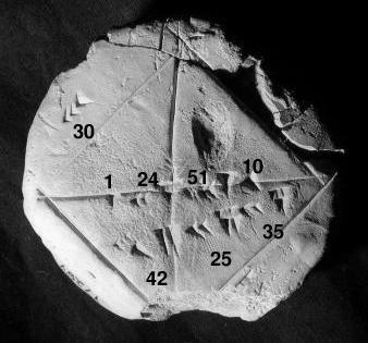
The Yale Babylonian Collection clay tablet YBC 7289 was created between 1800 BC and 1600 BC, showing ${\sqrt {2}}$ and ${\textstyle {\frac {\sqrt {2}}{2}}={\frac {1}{\sqrt {2}}}}$ respectively as 1;24,51,10 and 0;42,25,35 base 60 numbers on a square crossed by two diagonals. (1;24,51,10) base 60 corresponds to 1.41421296, which is correct to 5 decimal places (1.41421356...).

The Rhind Mathematical Papyrus is a copy from 1650 BC of an earlier Berlin Papyrus and other texts – possibly the Kahun Papyrus – that shows how the Egyptians extracted square roots by an inverse proportion method.

In Ancient India, the knowledge of theoretical and applied aspects of square and square root was at least as old as the Sulba Sutras, dated around 800–500 BC (possibly much earlier). A method for finding very good approximations to the square roots of 2 and 3 are given in the Baudhayana Sulba Sutra. Apastamba who was dated around 600 BCE has given a strikingly accurate value for ${\sqrt {2}}$ which is correct up to five decimal places as ${\textstyle 1+{\frac {1}{3}}+{\frac {1}{3\times 4}}-{\frac {1}{3\times 4\times 34}}}$. Aryabhata, in the Aryabhatiya (section 2.4), has given a method for finding the square root of numbers having many digits.

It was known to the ancient Greeks that square roots of positive integers that are not perfect squares are always irrational numbers: numbers not expressible as a ratio of two integers (that is, they cannot be written exactly as ${\frac {m}{n}}$, where m and n are integers). This is the theorem Euclid X, 9, almost certainly due to Theaetetus dating back to c. 380 BC. The discovery of irrational numbers, including the particular case of the square root of 2, is widely associated with the Pythagorean school. Although some accounts attribute the discovery to Hippasus, the specific contributor remains uncertain due to the scarcity of primary sources and the secretive nature of the brotherhood. It is exactly the length of the diagonal of a square with side length 1.

In the Chinese mathematical work Writings on Reckoning, written between 202 BC and 186 BC during the early Han dynasty, the square root is approximated by using an "excess and deficiency" method, which says to "...combine the excess and deficiency as the divisor; (taking) the deficiency numerator multiplied by the excess denominator and the excess numerator times the deficiency denominator, combine them as the dividend."

A symbol for square roots, written as an elaborate R, was invented by Regiomontanus (1436–1476). An R was also used for radix to indicate square roots in Gerolamo Cardano's Ars Magna.

According to historian of mathematics D.E. Smith, Aryabhata's method for finding the square root was first introduced in Europe by Cataneo—in 1546.

According to Jeffrey A. Oaks, Arabs used the letter jīm/ĝīm (ج), the first letter of the word "جذر" (variously transliterated as jaḏr, jiḏr, ǧaḏr or ǧiḏr, "root"), placed in its initial form (ﺟ) over a number to indicate its square root. The letter jīm resembles the present square root shape. Its usage goes as far as the end of the twelfth century in the works of the Moroccan mathematician Ibn al-Yasamin.

The symbol "√" for the square root was first used in print in 1525, in Christoph Rudolff's Coss.

Properties and uses

The graph of the function f(x) = √x, made up of half a parabola with a vertical directrix

The principal square root function $f(x)={\sqrt {x}}$ (usually just referred to as the "square root function") is a function that maps the set of nonnegative real numbers onto itself. In geometrical terms, the square root function maps the area of a square to its side length.

The square root of x is rational if and only if x is a rational number that can be represented as a ratio of two perfect squares. (See square root of 2 for proofs that this is an irrational number, and quadratic irrational for a proof for all non-square natural numbers.) The square root function maps rational numbers into algebraic numbers, the latter being a superset of the rational numbers).

For all real numbers x, $${\sqrt {x^{2}}}=\left|x\right|={\begin{cases}x,&{\text{if }}x\geq 0\\-x,&{\text{if }}x<0.\end{cases}}$$ (see absolute value).

For all nonnegative real numbers x and y, $${\sqrt {xy}}={\sqrt {x}}{\sqrt {y}}$$ and $${\sqrt {x}}=x^{1/2}.$$

The square root function is continuous for all nonnegative x, and differentiable for all positive x. If f denotes the square root function, whose derivative is given by: $$f'(x)={\frac {1}{2{\sqrt {x}}}}.$$

The Taylor series of ${\sqrt {1+x}}$ about x = 0 converges for |x| ≤ 1, and is given by

$${\sqrt {1+x}}=\sum _{n=0}^{\infty }{\frac {(-1)^{n}(2n)!}{(1-2n)(n!)^{2}(4^{n})}}x^{n}=1+{\frac {1}{2}}x-{\frac {1}{8}}x^{2}+{\frac {1}{16}}x^{3}-{\frac {5}{128}}x^{4}+\cdots ,$$

The square root of a nonnegative number is used in the definition of Euclidean norm (and distance), as well as in generalizations such as Hilbert spaces. It defines an important concept of standard deviation used in probability theory and statistics. It has a major use in the formula for roots of a quadratic equation; quadratic fields and rings of quadratic integers, which are based on square roots, are important in algebra and have uses in geometry. Square roots frequently appear in mathematical formulas elsewhere, as well as in many physical laws.

Square roots of positive integers

A positive number has two square roots, one positive, and one negative, which are opposite to each other. When talking of the square root of a positive integer, it is usually the positive square root that is meant.

The square roots of an integer are algebraic integers—more specifically quadratic integers.

The square root of a positive integer is the product of the roots of its prime factors, because the square root of a product is the product of the square roots of the factors. Since ${\textstyle {\sqrt {p^{2k}}}=p^{k},}$ only roots of those primes having an odd power in the factorization are necessary. More precisely, the square root of a prime factorization is $${\sqrt {p_{1}^{2e_{1}+1}\cdots p_{k}^{2e_{k}+1}p_{k+1}^{2e_{k+1}}\dots p_{n}^{2e_{n}}}}=p_{1}^{e_{1}}\dots p_{n}^{e_{n}}{\sqrt {p_{1}\dots p_{k}}}.$$

As decimal expansions

The square roots of the perfect squares (e.g., 0, 1, 4, 9, 16) are integers. In all other cases, the square roots of positive integers are irrational numbers, and hence have non-repeating decimals in their decimal representations. Decimal approximations of the square roots of the first few natural numbers are given in the following table.

n	${\sqrt {n}},$ truncated to 50 decimal places
0	0
1	1
2	1.41421356237309504880168872420969807856967187537694
3	1.73205080756887729352744634150587236694280525381038
4	2
5	2.23606797749978969640917366873127623544061835961152
6	2.44948974278317809819728407470589139196594748065667
7	2.64575131106459059050161575363926042571025918308245
8	2.82842712474619009760337744841939615713934375075389
9	3
10	3.16227766016837933199889354443271853371955513932521

As expansions in other numeral systems

As with before, the square roots of the perfect squares (e.g., 0, 1, 4, 9, 16) are integers. In all other cases, the square roots of positive integers are irrational numbers, and therefore have non-repeating digits in any standard positional notation system.

The square roots of small integers are used in both the SHA-1 and SHA-2 hash function designs to provide nothing up my sleeve numbers.

As periodic continued fractions

One of the most intriguing results from the study of irrational numbers as continued fractions was obtained by Joseph Louis Lagrange c. 1780. Lagrange found that the representation of the square root of any non-square positive integer as a continued fraction is periodic. That is, a certain pattern of partial denominators repeats indefinitely in the continued fraction. In a sense these square roots are the very simplest irrational numbers, because they can be represented with a simple repeating pattern of integers.

${\sqrt {2}}$	= [1; 2, 2, ...]
${\sqrt {3}}$	= [1; 1, 2, 1, 2, ...]
${\sqrt {4}}$	= [2]
${\sqrt {5}}$	= [2; 4, 4, ...]
${\sqrt {6}}$	= [2; 2, 4, 2, 4, ...]
${\sqrt {7}}$	= [2; 1, 1, 1, 4, 1, 1, 1, 4, ...]
${\sqrt {8}}$	= [2; 1, 4, 1, 4, ...]
${\sqrt {9}}$	= [3]
${\sqrt {10}}$	= [3; 6, 6, ...]
${\sqrt {11}}$	= [3; 3, 6, 3, 6, ...]
${\sqrt {12}}$	= [3; 2, 6, 2, 6, ...]
${\sqrt {13}}$	= [3; 1, 1, 1, 1, 6, 1, 1, 1, 1, 6, ...]
${\sqrt {14}}$	= [3; 1, 2, 1, 6, 1, 2, 1, 6, ...]
${\sqrt {15}}$	= [3; 1, 6, 1, 6, ...]
${\sqrt {16}}$	= [4]
${\sqrt {17}}$	= [4; 8, 8, ...]
${\sqrt {18}}$	= [4; 4, 8, 4, 8, ...]
${\sqrt {19}}$	= [4; 2, 1, 3, 1, 2, 8, 2, 1, 3, 1, 2, 8, ...]
${\sqrt {20}}$	= [4; 2, 8, 2, 8, ...]

The square bracket notation used above is a short form for a continued fraction. Written in the more suggestive algebraic form, the simple continued fraction for the square root of 11, [3; 3, 6, 3, 6, ...], looks like this: $${\sqrt {11}}=3+{\cfrac {1}{3+{\cfrac {1}{6+{\cfrac {1}{3+{\cfrac {1}{6+{\cfrac {1}{3+\ddots }}}}}}}}}}$$

where the two-digit pattern {3, 6} repeats over and over again in the partial denominators. Since 11 = 3² + 2, the above is also identical to the following generalized continued fractions:

$${\sqrt {11}}=3+{\cfrac {2}{6+{\cfrac {2}{6+{\cfrac {2}{6+{\cfrac {2}{6+{\cfrac {2}{6+\ddots }}}}}}}}}}=3+{\cfrac {6}{20-1-{\cfrac {1}{20-{\cfrac {1}{20-{\cfrac {1}{20-{\cfrac {1}{20-\ddots }}}}}}}}}}.$$

Computation

Main article: Methods of computing square roots

Square roots of positive numbers are not in general rational numbers, and so cannot be written as a terminating or recurring decimal expression. Therefore in general any attempt to compute a square root expressed in decimal form can only yield an approximation, though a sequence of increasingly accurate approximations can be obtained.

Most pocket calculators have a square root key. Computer spreadsheets and other software are also frequently used to calculate square roots. Pocket calculators typically implement efficient routines, such as the Newton's method (frequently with an initial guess of 1), to compute the square root of a positive real number. When computing square roots with logarithm tables or slide rules, one can exploit the identities $${\sqrt {a}}=e^{(\ln a)/2}=10^{(\log _{10}a)/2},$$ where ln and log₁₀ are the natural and base-10 logarithms.

By trial-and-error, one can square an estimate for ${\sqrt {a}}$ and raise or lower the estimate until it agrees to sufficient accuracy. For this technique it is prudent to use the identity $$(x+c)^{2}=x^{2}+2xc+c^{2},$$ as it allows one to adjust the estimate x by some amount c and measure the square of the adjustment in terms of the original estimate and its square.

The most common iterative method of square root calculation by hand is known as the "Babylonian method" or "Heron's method" after the first-century Greek philosopher Heron of Alexandria, who first described it. The method uses the same iterative scheme as the Newton–Raphson method yields when applied to the function y = f(x) = x² − a, using the fact that its slope at any point is dy/dx = f′(x) = 2x, but predates it by many centuries. The algorithm is to repeat a simple calculation that results in a number closer to the actual square root each time it is repeated with its result as the new input. The motivation is that if x is an overestimate to the square root of a nonnegative real number a then a/x will be an underestimate and so the average of these two numbers is a better approximation than either of them. However, the inequality of arithmetic and geometric means shows this average is always an overestimate of the square root (as noted below), and so it can serve as a new overestimate with which to repeat the process, which converges as a consequence of the successive overestimates and underestimates being closer to each other after each iteration. To find x:

1. Start with an arbitrary positive start value x. The closer to the square root of a, the fewer the iterations that will be needed to achieve the desired precision.
2. Replace x by the average (x + a/x) / 2 between x and a/x.
3. Repeat from step 2, using this average as the new value of x.

That is, if an arbitrary guess for ${\sqrt {a}}$ is x₀, and x_{n + 1} = (x_n + a/x_n) / 2, then each x_n is an approximation of ${\sqrt {a}}$ which is better for large n than for small n. If a is positive, the convergence is quadratic, which means that in approaching the limit, the number of correct digits roughly doubles in each next iteration. If a = 0, the convergence is only linear; however, ${\sqrt {0}}=0$ so in this case no iteration is needed.

Using the identity $${\sqrt {a}}=2^{-n}{\sqrt {4^{n}a}},$$ the computation of the square root of a positive number can be reduced to that of a number in the range [1, 4). This simplifies finding a start value for the iterative method that is close to the square root, for which a polynomial or piecewise-linear approximation can be used.

The time complexity for computing a square root with n digits of precision is equivalent to that of multiplying two n-digit numbers.

Another useful method for calculating the square root is the shifting nth root algorithm, applied for n = 2.

The name of the square root function varies from programming language to programming language, with sqrt (often pronounced "squirt" ) being common, used in C and derived languages like C++, JavaScript, PHP, and Python.

Square roots of negative and complex numbers

First leaf of the complex square root

Second leaf of the complex square root

Using the Riemann surface of the square root, it is shown how the two leaves fit together

The square of any positive or negative number is positive, and the square of 0 is 0. Therefore, no negative number can have a real square root. However, it is possible to work with a more inclusive set of numbers, called the complex numbers, that does contain solutions to the square root of a negative number. This is done by introducing a new number, denoted by i (sometimes by j, especially in the context of electricity where i traditionally represents electric current) and called the imaginary unit, which is defined such that i² = −1. Using this notation, we can think of i as the square root of −1, but we also have (−i)² = i² = −1 and so −i is also a square root of −1. By convention, the principal square root of −1 is i, or more generally, if x is any nonnegative number, then the principal square root of −x is $${\sqrt {-x}}=i{\sqrt {x}}.$$

The right side (as well as its negative) is indeed a square root of −x, since $$(i{\sqrt {x}})^{2}=i^{2}({\sqrt {x}})^{2}=(-1)x=-x.$$

For every non-zero complex number z there exist precisely two numbers w such that w² = z: the principal square root of z (defined below), and its negative.

Principal square root of a complex number

Geometric representation of the 2nd to 6th roots of a complex number z, in polar form re^iφ  where r = |z | and φ = arg z. If z is real, φ = 0 or π. Principal roots are shown in black.

To find a definition for the square root that allows us to consistently choose a single value, called the principal value, we start by observing that any complex number $x+iy$ can be viewed as a point in the plane, $(x,y),$ expressed using Cartesian coordinates. The same point may be reinterpreted using polar coordinates as the pair $(r,\varphi ),$ where $r\geq 0$ is the distance of the point from the origin, and $\varphi$ is the angle that the line from the origin to the point makes with the positive real ($x$) axis. In complex analysis, the location of this point is conventionally written $re^{i\varphi }.$ If $$z=re^{i\varphi }{\text{ with }}-\pi <\varphi \leq \pi ,$$ then the principal square root of $z$ is defined to be the following: $${\sqrt {z}}={\sqrt {r}}e^{i\varphi /2}.$$ The principal square root function is thus defined using the non-positive real axis as a branch cut. If $z$ is a non-negative real number (which happens if and only if $\varphi =0$) then the principal square root of $z$ is ${\sqrt {r}}e^{i(0)/2}={\sqrt {r}};$ in other words, the principal square root of a non-negative real number is just the usual non-negative square root. It is important that $-\pi <\varphi \leq \pi$ because if, for example, $z=-2i$ (so $\varphi =-\pi /2$) then the principal square root is $${\sqrt {-2i}}={\sqrt {2e^{i\varphi }}}={\sqrt {2}}e^{i\varphi /2}={\sqrt {2}}e^{i(-\pi /4)}=1-i$$ but using ${\tilde {\varphi }}:=\varphi +2\pi =3\pi /2$ would instead produce the other square root ${\sqrt {2}}e^{i{\tilde {\varphi }}/2}={\sqrt {2}}e^{i(3\pi /4)}=-1+i=-{\sqrt {-2i}}.$

The principal square root function is holomorphic everywhere except on the set of non-positive real numbers (on strictly negative reals it is not even continuous). The above Taylor series for ${\sqrt {1+x}}$ remains valid for complex numbers $x$ with $|x|<1.$

The above can also be expressed in terms of trigonometric functions: $${\sqrt {r\left(\cos \varphi +i\sin \varphi \right)}}={\sqrt {r}}\left(\cos {\frac {\varphi }{2}}+i\sin {\frac {\varphi }{2}}\right).$$

Algebraic formula

The square roots of i

When the number is expressed using its real and imaginary parts, the following formula can be used for the principal square root:

$${\sqrt {x+iy}}={\sqrt {{\tfrac {1}{2}}{\bigl (}{\sqrt {\textstyle x^{2}+y^{2}}}+x{\bigr )}}}+i\operatorname {sgn}(y){\sqrt {{\tfrac {1}{2}}{\bigl (}{\sqrt {\textstyle x^{2}+y^{2}}}-x{\bigr )}}},$$

where sgn(y) = 1 if y ≥ 0 and sgn(y) = −1 otherwise. In particular, the imaginary parts of the original number and the principal value of its square root have the same sign. The real part of the principal value of the square root is always nonnegative.

For example, the principal square roots of ±i are given by:

$${\sqrt {i}}={\frac {1+i}{\sqrt {2}}},\qquad {\sqrt {-i}}={\frac {1-i}{\sqrt {2}}}.$$

Notes

In the following, the complex z and w may be expressed as:

• $z=|z|e^{i\theta _{z}}$
• $w=|w|e^{i\theta _{w}}$

where $-\pi <\theta _{z}\leq \pi$ and $-\pi <\theta _{w}\leq \pi$.

Because of the discontinuous nature of the square root function in the complex plane, the following laws are not true in general.

• ${\sqrt {zw}}={\sqrt {z}}{\sqrt {w}}$
  Counterexample for the principal square root: z = −1 and w = −1
  This equality is valid only when $-\pi <\theta _{z}+\theta _{w}\leq \pi$
• ${\frac {\sqrt {w}}{\sqrt {z}}}={\sqrt {\frac {w}{z}}}$
  Counterexample for the principal square root: w = 1 and z = −1
  This equality is valid only when $-\pi <\theta _{w}-\theta _{z}\leq \pi$
• ${\sqrt {z^{*}}}=\left({\sqrt {z}}\right)^{*}$
  Counterexample for the principal square root: z = −1)
  This equality is valid only when $\theta _{z}\neq \pi$

A similar problem appears with other complex functions with branch cuts, e.g., the complex logarithm and the relations logz + logw = log(zw) or log(z^*) = log(z)^* which are not true in general.

Wrongly assuming one of these laws underlies several faulty "proofs", for instance the following one showing that −1 = 1: $${\begin{aligned}-1&=i\cdot i\\&={\sqrt {-1}}\cdot {\sqrt {-1}}\\&={\sqrt {\left(-1\right)\cdot \left(-1\right)}}\\&={\sqrt {1}}\\&=1.\end{aligned}}$$

The third equality cannot be justified (see invalid proof). It can be made to hold by changing the meaning of √ so that this no longer represents the principal square root (see above) but selects a branch for the square root that contains ${\sqrt {1}}\cdot {\sqrt {-1}}.$ The left-hand side becomes either $${\sqrt {-1}}\cdot {\sqrt {-1}}=i\cdot i=-1$$ if the branch includes +i or $${\sqrt {-1}}\cdot {\sqrt {-1}}=(-i)\cdot (-i)=-1$$ if the branch includes −i, while the right-hand side becomes $${\sqrt {\left(-1\right)\cdot \left(-1\right)}}={\sqrt {1}}=-1,$$ where the last equality, ${\sqrt {1}}=-1,$ is a consequence of the choice of branch in the redefinition of √.

nth roots and polynomial roots

The definition of a square root of $x$ as a number $y$ such that $y^{2}=x$ has been generalized in the following way.

A cube root of $x$ is a number $y$ such that $y^{3}=x$; it is denoted ${\sqrt[{3}]{x}}.$

If n is an integer greater than two, a n-th root of $x$ is a number $y$ such that $y^{n}=x$; it is denoted ${\sqrt[{n}]{x}}.$

Given any polynomial p, a root of p is a number y such that p(y) = 0. For example, the nth roots of x are the roots of the polynomial (in y) $y^{n}-x.$

Abel–Ruffini theorem states that, in general, the roots of a polynomial of degree five or higher cannot be expressed in terms of nth roots.

Square roots of matrices and operators

Main article: Square root of a matrix

See also: Square root of a 2 by 2 matrix

If A is a positive-definite matrix or operator, then there exists precisely one positive definite matrix or operator B with B² = A; we then define A^1/2 = B. In general matrices may have multiple square roots or even an infinitude of them. For example, the 2 × 2 identity matrix has an infinity of square roots, though only one of them is positive definite.

In integral domains, including fields

Each element of an integral domain has no more than 2 square roots. The difference of two squares identity u² − v² = (u − v)(u + v) is proved using the commutativity of multiplication. If u and v are square roots of the same element, then u² − v² = 0. Because there are no zero divisors this implies u = v or u + v = 0, where the latter means that two roots are additive inverses of each other. In other words if an element a square root u of an element a exists, then the only square roots of a are u and −u. The only square root of 0 in an integral domain is 0 itself.

In a field of characteristic 2, an element either has one square root or does not have any at all, because each element is its own additive inverse, so that −u = u. If the field is finite of characteristic 2 then every element has a unique square root. In a field of any other characteristic, any non-zero element either has two square roots, as explained above, or does not have any.

Given an odd prime number p, let q = p^e for some positive integer e. A non-zero element of the field F_q with q elements is a quadratic residue if it has a square root in F_q. Otherwise, it is a quadratic non-residue. There are (q − 1)/2 quadratic residues and (q − 1)/2 quadratic non-residues; zero is not counted in either class. The quadratic residues form a group under multiplication. The properties of quadratic residues are widely used in number theory.

In rings in general

Unlike in an integral domain, a square root in an arbitrary (unital) ring need not be unique up to sign. For example, in the ring $\mathbb {Z} /8\mathbb {Z}$ of integers modulo 8 (which is commutative, but has zero divisors), the element 1 has four distinct square roots: ±1 and ±3.

Another example is provided by the ring of quaternions $\mathbb {H} ,$ which has no zero divisors, but is not commutative. Here, the element −1 has infinitely many square roots, including ±i, ±j, and ±k. In fact, the set of square roots of −1 is exactly $$\{ai+bj+ck\mid a^{2}+b^{2}+c^{2}=1\}.$$

A square root of 0 is either 0 or a zero divisor. Thus in rings where zero divisors do not exist, it is uniquely 0. However, rings with zero divisors may have multiple square roots of 0. For example, in $\mathbb {Z} /n^{2}\mathbb {Z} ,$ any multiple of n is a square root of 0.

Geometric construction of the square root

Constructing the length $x={\sqrt {a}}$, given the $a$ and the unit length

The Spiral of Theodorus up to the triangle with a hypotenuse of √4

The square root of a positive number is usually defined as the side length of a square with the area equal to the given number. But the square shape is not necessary for it: if one of two similar planar Euclidean objects has the area a times greater than another, then the ratio of their linear sizes is ${\sqrt {a}}$.

A square root can be constructed with a compass and straightedge. In his Elements, Euclid (fl. 300 BC) gave the construction of the geometric mean of two quantities in two different places: Proposition II.14 and Proposition VI.13. Since the geometric mean of a and b is ${\sqrt {ab}}$, one can construct ${\sqrt {a}}$ simply by taking b = 1.

The construction is also given by Descartes in his La Géométrie, see figure 2 on page 2. However, Descartes made no claim to originality and his audience would have been quite familiar with Euclid.

Euclid's second proof in Book VI depends on the theory of similar triangles. Let AHB be a line segment of length a + b with AH = a and HB = b. Construct the circle with AB as diameter and let C be one of the two intersections of the perpendicular chord at H with the circle and denote the length CH as h. Then, using Thales' theorem and, as in the proof of Pythagoras' theorem by similar triangles, triangle AHC is similar to triangle CHB (as indeed both are to triangle ACB, though we don't need that, but it is the essence of the proof of Pythagoras' theorem) so that AH:CH is as HC:HB, i.e. a/h = h/b, from which we conclude by cross-multiplication that h² = ab, and finally that $h={\sqrt {ab}}$. When marking the midpoint O of the line segment AB and drawing the radius OC of length (a + b)/2, then clearly OC > CH, i.e. ${\textstyle {\frac {a+b}{2}}\geq {\sqrt {ab}}}$ (with equality if and only if a = b), which is the arithmetic–geometric mean inequality for two variables and, as noted above, is the basis of the Ancient Greek understanding of "Heron's method".

Another method of geometric construction uses right triangles and induction: ${\sqrt {1}}$ can be constructed, and once ${\sqrt {x}}$ has been constructed, the right triangle with legs 1 and ${\sqrt {x}}$ has a hypotenuse of ${\sqrt {x+1}}$. Constructing successive square roots in this manner yields the Spiral of Theodorus depicted above.

See also

• Apotome (mathematics)
• Cube root
• Functional square root
• Integer square root
• Nested radical
• Nth root
• Root of unity
• Solving quadratic equations with continued fractions
• Square-root sum problem
• Square root principle
• Quantum gate § Square root of NOT gate (√NOT)

References

• Dauben, Joseph W. (2007). "Chinese Mathematics I". In Katz, Victor J. (ed.). The Mathematics of Egypt, Mesopotamia, China, India, and Islam. Princeton: Princeton University Press. ISBN 978-0-691-11485-9.
• Gel'fand, Izrael M.; Shen, Alexander (1993). Algebra (3rd ed.). Birkhäuser. p. 120. ISBN 0-8176-3677-3.
• Joseph, George (2000). The Crest of the Peacock. Princeton: Princeton University Press. ISBN 0-691-00659-8.
• Smith, David (1958). History of Mathematics. Vol. 2. New York: Dover Publications. ISBN 978-0-486-20430-7.
• Selin, Helaine (2008), Encyclopaedia of the History of Science, Technology, and Medicine in Non-Western Cultures, Springer, Bibcode:2008ehst.book.....S, ISBN 978-1-4020-4559-2.

External links

• Algorithms, implementations, and more – Paul Hsieh's square roots webpage
• How to manually find a square root
• AMS Featured Column, Galileo's Arithmetic by Tony Philips – includes a section on how Galileo found square roots